Random Forest Machine Learning in R, Python and SQL – Part 2

This is the second part of a two-article series on using Random Forest in R, Python and SQL. In the first article, Random Forest was introduced, with details of how it works. Examples of using Random Forest were given using the R language. This article builds upon what was covered in the first part, giving examples of building and using Random Forest models using Python and Oracle 18c Database.

Check out the first article here.

The same data set used in the first article will be used in this article, for the Python language and Oracle 18cDatabase. This will allow you to easily understand all components and to be able to migrate between the languages.

Random Forest in Python

Python has become one of the most popular languages for machine learning over the past year. There are lots of reasons for this: Python is easy to learn, there are lots of new packages available for it (particularly for data science), it can be used to develop production applications, and it is easy to integrate into existing production systems.

Before you can start using Random Forest in Python, there are a number of packages/libraries you need to install. These include scikit-Learn (the main machine learning package currently available), along with some of the more typical data processing packages encountered in data science projects. To install these packages run the following commands in a command line shell/window.

pip3 install -U scikit-learn

pip3 install -U numpy

pip3 install -U scipy

pip3 install -U matplotlib

pip3 install -U pandas

The following Python code follows the same flow as what was shown in the R sample code in the first article, beginning with loading the data set into a panda in our Python environment. This panda object (just like a dataframe in R and a spreadsheet) can be used to inspect and gather some initial statistics about the data. Pandas are great for doing this and have a large number of statistical features built in.

# read the data set into the panda

import pandas as pd

Bank_df = pd.read_csv('/users/brendan.tierney/Downloads/bank-additional/bank-additional-full.csv', sep=";")

# display the data

Bank_df

# explore the data

Bank_df.info()

# gather basic statistics about each column.

#  very like summary function in R

Bank_df.describe()

# number of rows and columns

Bank_df.shape

# list the column names

Bank_df.columns

As with all data sets, they will require some formatting and cleaning up before they can be inputted into the machine learning algorithms. Depending on the maturity of the language, additional coding may be required. This is the case with Python, where data preparation is needed to format the target attribute and columns containing character strings.

The target variable has a label of ‘y’, which isn’t really meaningful. Additionally, it consists of character strings of ‘no’ or ‘yes’. This needs to be converted into numeric representation, with zero representing the ‘no’ values and one representing the ‘yes’ values. The pandas function factorize can be used to do this, and is assigned to a new column called TARGET. The original ‘y’ column can now be removed from the data set.

# recode reponse variable into 1/0

Bank_df2 = Bank_df

Bank_df2['TARGET'] = pd.factorize(Bank_df2['y'])[0]

# remove the 'y' column

Bank_df2 = Bank_df2.drop('y', 1)

The machine learning algorithms in Python (and other languages) like to have all the data represented as numbers. But in most data sets (and in our Bank data set) some columns will contain character strings. These are commonly referred to as categorical variables. In Python we need to convert these into a number of additional columns that will contain a zero or a one depending on the value in the original variable. For example, the ‘marital’ column contains three values (‘single’, ‘married’, ‘divorced’). A technique call one-hot coding is used to cover this single column into three columns called ‘marital_divorced’, ‘marital_married’, ‘marital_single’. If a record has a value of ‘married’ then a number one will be stored in the ‘marital_married’ column and a zero in the ‘marital_single’ and ‘marital_divorced’ columns.

# Perform one-hot encoding for categorical features.

# These are   job, marital, education, default, housing, load, contact, month, day_of_week, poutcome

# One-hot encode the data using pandas get_dummies

Bank_df3 = pd.get_dummies(Bank_df2, dummy_na=True)

Bank_df3.columns

The above code uses the pandas function get_dummies to perform the one-hot coding.

The data set is now prepared for input to the machine learning algorithm. Before we do that, the data set needs to be divided into training (70%) and testing (30%) data sets. There are several approaches to do this, but the following example uses the function available in scikit-learn to split the data sets.

# check out alternative training/test split method with scikitLearn

from sklearn.model_selection import train_test_split

training_sample2, testing_sample2 = train_test_split(Bank_df3, test_size=0.3, random_state=42)

print("Training data set size = ", len(training_sample2))

print("Testing data set size = ", len(testing_sample2))

The final step in preparing the data is to divide and separate the Target variable and the input variables. These need to separated and fed into the algorithm as separate inputs.

# list the attributes needed for inputs

# Labels are the values we want to predict i.e. target variable

train_labels = np.array(training_sample2['TARGET'])

# remove the target variable from the data set. axis=1 means drop column

train_features = training_sample2.drop('TARGET', axis=1)

training_sample2 = train_features

# Saving feature names for later use

train_feature_list = list(train_features.columns)

# Convert to numpy array

train_features = np.array(train_features)

These can now be inputted to the algorithm and the Random Forest model is created. This example is using the classification version of the algorithm. If the data set and problem was for regression, the RandomForestRegression algorithm could be used.

# setup Random Forest algorithm

# Import the model we are using

#from sklearn.ensemble import RandomForestRegressor

from sklearn.ensemble import RandomForestClassifier

# Instantiate model with 50 decision trees

rf = RandomForestClassifier(n_estimators = 50, random_state = 42)

# create or fit the model

# train the model on training sample data set

rf.fit(train_features, train_labels);

The following commands inspect the properties of the created model.

# list decision trees estimators

print(rf.estimators_)

print('——————–')

print('Num of classes')

print(rf.n_classes_)

print('——————–')

print('Class labels')

print(rf.classes_)

print('——————–')

print('Num of features when fit is perform')

print(rf.n_features_)

print('——————–')

print('Num of outputs when fit is performed')

print(rf.n_outputs_)

print('——————–')

print('Feature Importance')

print(rf.feature_importances_)

To evaluate the model the scikit-learn package has a wide range of functions.  The following example uses tenfold cross validation to test and evaluate the model and calculate its accuracy.

from sklearn.model_selection import cross_validate

accuracy = cross_validate(rf, test_features, test_labels, cv=10)['test_score']

print('The accuracy is: ',sum(accuracy)/len(accuracy)*100,'%')

The accuracy is:  91.00104692394183 %

And create the ROC chart.

# plot ROC chart

plt.title('Receiver Operating Characteristic')

plt.plot(false_positive_rate, true_positive_rate, 'b',

label='AUC = %0.2f'% roc_auc)

plt.legend(loc='lower right')

plt.plot([0,1],[0,1],'r–')

plt.xlim([-0.1,1.2])

plt.ylim([-0.1,1.2])

plt.ylabel('True Positive Rate')

plt.xlabel('False Positive Rate')

plt.show()    # see figure 5

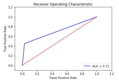
Figure 5: Python ROC chart

To inspect and chart the important variables in the data set that are dominant in making the predictions we can:

# Get numerical feature importances

import matplotlib.pyplot as plt

%matplotlib inline

importances = list(rf.feature_importances_)

# Set the style

plt.style.use('fivethirtyeight')

plt.figure(figsize=(16,8))

# list of x locations for plotting

x_values = list(range(len(importances)))

# Make a bar chart

plt.bar(x_values, importances, orientation = 'vertical')

# Tick labels for x axis

plt.xticks(x_values, feature_list, rotation='vertical')

# Axis labels and title

plt.ylabel('Importance'); plt.xlabel('Variable'); plt.title('Variable Importances')  # See Figure 6

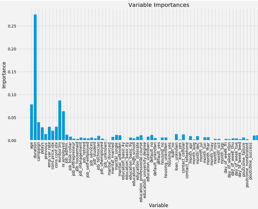
Figure 6 : Attribute Importance Chart

Random Forest in Oracle 18c

Over the past few years more databases are having machine learning incorporated into their core engines. The idea behind this relates to “bring the algorithms to the data instead of the data to the algorithms”. Many of the commercial database vendors, and some open source databases, now have many of the most commonly used machine learning algorithms built into them.

The examples used in this section are based on the implementation of Random Forest available in Oracle 18c Enterprise Edition. You can try this out for yourself on the Oracle Cloud (cloud.oracle.com), or by downloading and installing the Oracle 18c Database (either Enterprise Edition or XE edition), or by downloading a virtual machine with everything already installed and configured for you (http://www.oracle.com/technetwork/community/developer-vm/index.html)

The first step is to load the data set into a table in the database. Many of the SQL client tools have features that inspect a CSV file and will then create a table based on the structure of the data and then load the data into it. In the examples shown below the data set was loaded into a table called BANKING_ADDITIONAL.

The next step is to set up the training and testing data sets. This can be done by random sampling the data set in the BANKING_ADDITIONAL table. When the original data set was imported into a table called BANKING_ADDITIONAL, some of the variables were renamed to make them compatible with database conventions. The data set does not contain a case identifier. An artificial one (called CUST_ID) was created and a database record identifier was used to populate this. This is useful for creating the training and test data sets.

create or replace view bank_train_v

as select * from banking_additional

where ora_hash(cust_id,99) <= 70;

create or replace view bank_test_v

as select * from banking_additional

where ora_hash(cust_id,99) > 70;

Next, a table is needed to contain the parameter settings for the Random Forest algorithm. The table in the following code segment only defines the default parameters needed to run the algorithm.

— create the settings table for a Random Forest model

CREATE TABLE demo_RF_settings

( setting_name  VARCHAR2(30),

  setting_value VARCHAR2(4000));

— insert the settings records for a Neural Network

— ADP is turned on. By default ADP is turned off.

BEGIN

  INSERT INTO demo_RF_settings (setting_name, setting_value)

  values (dbms_data_mining.algo_name,

          dbms_data_mining.algo_random_forest);

  INSERT INTO demo_neural_network_settings (setting_name, setting_value)

  VALUES (dbms_data_mining.prep_auto, dbms_data_mining.prep_auto_on);

END;

The additional parameters include:

• Setting the sampling rate
• Setting the depth of the decision trees
• Setting the number of decision trees to create

The CREATE_MODEL function can be used to create the model and store it in the database. The example data set is a classification problem, which defined in this function. If it was a regression problem then it could be defined here also.

BEGIN

   DBMS_DATA_MINING.CREATE_MODEL(

      model_name          => 'DEMO_RF_MODEL',

      mining_function     => dbms_data_mining.classification,

      data_table_name     => 'bank_train_v',

      case_id_column_name => 'cust_id',

      target_column_name  => 'target',

      settings_table_name => 'demo_rf_settings');

END;

All of this took less than one second to run on the database I was running.

The default number of decision trees created is 20. This can be changed in the settings table by adding a record for the variable FOR_NTREES.

When the model is applied to the testing data set, we get an overall model accuracy of 91%.

The Random Forest model can be used to label new data by using the SQL functions PREDICTION, PREDICTION_PROBABILITY. The following gives an example of this.

SELECT cust_id, target,

       prediction(DEMO_RF_MODEL USING *)  predicted_value,

       prediction_probability(DEMO_RF_MODEL USING *) probability

FROM   bank_test_v;

Summary

Random Forest is a powerful machine learning algorithm, allowing you to create very accurate and reliable models. All the main machine learning languages come with Random Forest as a core algorithm, and it has been widely used in many industries to address and solve important business use cases, such as fraud, churn, target marketing, special offers, insurance payments, etc. Examples have been given in R, Python and in Oracle 18c. You can see that there are different levels of work involved in preparing and using the algorithm and the generated model. There are definite steps being taken to automate the boring stuff; that is, to automate the more routine steps. This is evident in R and Oracle 18c, whereas Python needed a lot more coding. Although, R ,and Python have good charting features, and although SQL lacks this without using another tool, having the model and processing in the database involves less data movement and the model works on the data using the scalability and power of the database server. Each language has its advantages and disadvantages.