Most of us have probably seen a game show where the competitor has the option of asking the audience for help with answering a question. The game show host will read out the question and all members of the audience will then vote for what they think is the correct answer. The competitor can then make an informed answer that is based on how everyone has voted. This is a kind of crowd sourcing a solution, and this is the basics of how the machine learning algorithm Random Forest works. Random Forest is an ensemble machine learning algorithm that create many tens or hundreds of decision tree models and then uses all of these to make a prediction.
This two-article series will give an explanation of how the Random Forest algorithm works, from how it builds a model based on an input data set, to how the model works for making a prediction. Examples will be given on how to use Random Forest using popular machine learning algorithms including R, Python, and SQL. Using the in-database implementation of Random Forest accessible using SQL allows for DBAs, developers, analysts and citizen data scientists to quickly and easily build these models into their production applications.
This first article covers some of the details of how Random Forest works and then illustrates how to use the R language to create and use Random Forest models.
The second article will look at how you can build Random Forest models in Python and in Oracle 18c Database. Make sure to check out that article.
What is Random Forest?
Random Forest is known as an ensemble machine learning technique that involves the creation of hundreds of decision tree models. These hundreds of models are used to label or score new data by evaluating each of the decision trees and then determining the outcome based on the majority result from all the decision trees. Just like in the game show. The combining of a number of different ways of making a decision can result in a more accurate result or prediction.
Random Forest models can be used for classification and regression types of problems, which form the majority of machine learning systems and solutions. For classification problems, this is where the target variable has either a binary value or a small number of defined values. For classification problems the Random Forest model will evaluate the predicted value for each of the decision trees in the model. The final predicted outcome will be the majority vote for all the decision trees. For regression problems the predicted value is numeric and on some range or scale. For example, we might want to predict a customer’s lifetime value (LTV), or the potential value of an insurance claim, etc. With Random Forest, each decision tree will make a prediction of this numeric value. The algorithm will then average these values for the final predicted outcome.
Under the hood, Random Forest is a collection of decision trees. Although decision trees (Figure 1) are a popular algorithm for machine learning, they can have a tendency to over fit the model. This can lead higher than expected errors when predicting unseen data. It also gives just one possible way of representing the data and being able to derive a possible predicted outcome.
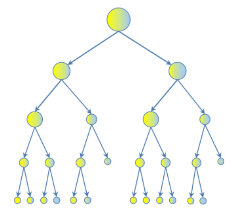
Figure 1 – Decision Tree
Random Forest (Figure 2) on the other hand relies of the predicted outcomes from many different decision trees, each of which is built in a slightly different way. It is an ensemble technique that combines the predicted outcomes from each decision tree to give one answer. Typically, the number of trees created by the Random Forest algorithm is defined by a parameter setting, and in most languages this can default to 100+ or 200+ trees.
The Random Forest algorithm has three main features:
– It uses a method called bagging to create different subsets of the original training data
– It will randomly section different subsets of the features/attributes and build the decision tree based on this subset
– By creating many different decision trees, based on different subsets of the training data and different subsets of the features, it will increase the probability of capturing all possible ways of modeling the data
For each decision tree produced, the algorithm will use a measure, such as the Gini index , to select the attributes to split on at each node of the decision tree.
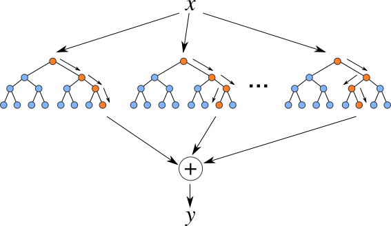
Figure 2 – Example of Random Forest
Care is needed with considering Random Forest for production use. Because of the high number of decision trees to evaluate for each individual record or prediction, the time to make the prediction might appear to be slow in comparison to models created using other machine learning algorithms. You need to consider the time for scoring/labeling the data versus the accuracy of the predictions. To minimize this issue, the number of trees in the Random Forest model can be reduced to tens of trees instead of hundreds.
The following sections will illustrate how a Random Forest machine learning model can be create in three of the most popular languages used by data scientists. Each example will use the same data set and will follow the steps of loading the data set, creating the training and test data sets, and the creation of the Random Forest model; and some simple evaluation and accuracy metrics will be created.
The Data Set
The data set used in the following examples is the Bank Marketing data set. This is available on the UCI Machine Learning Repository (https://archive.ics.uci.edu/ml/datasets/Bank+Marketing ). The data set is from a Portugese Bank that wanted to use machine learning to predict what customers are likely to open a new type of bank account. The original paper written about this data set and their initial work can be found at http://media.salford-systems.com/video/tutorial/2015/targeted_marketing.pdf.
Random Forests in R
The following code illustrates the creating of a Random Forest model using R for our Banking Dataset. It uses therandomForest and ROCR packages. You can use the following command to install these packages.
install.packages(“randomForest”, “ROCR”
The following code goes through the following steps
- Load the randomForest package
- Loads the Banking database from a CSV file into a data frame
- Inspects the dataframe and generates some basic statistics
library(randomForest)

# load the data set from CSV file
BankData <- read.csv(file="/Users/brendan.tierney/Downloads/bank-additional/bank-additional-full.csv", header=TRUE, sep=";")

# Let us investage this dataset and gather some informations and statistics
head(BankData)
ncol(BankData)
nrow(BankData)
names(BankData)
str(BankData)
dim(BankData)
summary(BankData)
Next, the training and testing data sets are created. Seventy percent of the data is used for training the Random Forest model and the remaining thirty percent is kept for testing the model.
# Set the sample size to be 40% of the full data set
# The Testing data set will have 30% of the records
# The Training data set will have 70% of the records
SampleSize <- nrow(BankData)*0.30

# Create an index of records for the Sample
Index_Sample <- sample(1:nrow(BankData), SampleSize)
group <- as.integer(1:nrow(BankData) %in% Index_Sample)

# Create a partitioned data set of those records not selected to be in sample
Training_Sample <- BankData[group==FALSE,]

# Get the number of records in the Training Sample data set
nrow(Training_Sample)

# Create a partitioned data set of those records who were selected to be in the sample
Testing_Sample <- BankData[group==TRUE,]

# Get the number of records in the Testing Sample data set
nrow(Testing_Sample)
The read.csv function converted all string and categorical variables to factors. The data set should also be checked to see if any numeric variables should be converted to factors. The data in our data set can be used as it is without any additional changes.
The model can now be generated, and the model object is inspected to see the metadata generated for the model. A random seed can be assigned to the algorithm or use the default.
# set the random seed
# set.seed(42)
# generate/fit the model with 50 trees
rf_model <- randomForest(y~., data=Training_Sample, ntree=50)

# print basic model details, including confusion matrix
rf_model
names(rf_model)
rf_model$call
rf_model$type
rf_model$terms
rf_model$ntree
rf_model$mtry
rf_model$classes
rf_model$DOP
rf_model$confusion
rf_model$RFOPKG
summary(rf_model)
The model can give us many useful insights on the data and each column/feature in the dataset. Attribute importance is one such insight, informing us of what columns/features are of most important for determining the predicted outcome, along with the ranking of these columns/features.
#Evaluate variable importance
importance(rf_model)
MeanDecreaseGini
age 416.00613
job 355.71471
marital 114.61366
education 262.59905
default 39.92922
housing 92.42560
loan 74.33467
contact 47.15442
month 181.98392
day_of_week 254.27931
duration 1683.89729
campaign 203.14304
pdays 206.34775
previous 78.76455
poutcome 113.34445
emp.var.rate 128.64761
cons.price.idx 105.80007
cons.conf.idx 196.99971
euribor3m 575.27280
nr.employed 294.29843
varImpPlot(rf_model)
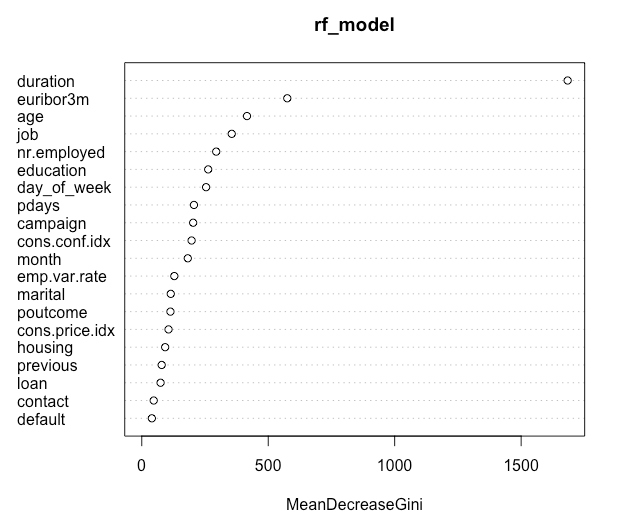
Figure 3 – Attribute Importance plot
The higher the value of mean decrease accuracy or mean decrease Gini score, the higher the importance of the variable in the model. In the plot shown above (Figure 3), Account Balance is the most important variable.
After the model has been generated, it can be used to make predictions for the Testing data set. This is an unseen data set and is typically used to test or evaluate the model.
# Score/label new data set = Testing Data set
RF_scored <- predict(rf_model, newdata=Testing_Sample, type="response")

# add the predicted value to the dataset
RF_scored2 <- cbind(Testing_Sample, RF_scored)

# create cross tab table on actual values vs predicted values i.e. confusion matrix
table(RF_scored2$y, RF_scored2$RF_scored)
no yes
no 10588 395
yes 662 711
You can see that the model has a very high overall accuracy rate. It is extremely good at predicting where the target column is ‘no’, but less accurate at prediction ‘yes’ values. Perhaps this is something that is worth exploring more; additional models could be built to get a better accuracy for the ‘yes’ values.
The prediction probabilities can also be predicted. This gives an indication of how strong of a prediction was made. Two probabilities are produced, one for each of the values in the target column.
The next step that is typically performed is to create the ROC chart. This is a good way of visualizing how effective the model is based on the rate of false positives vs. the rate of true positives.
To generate the ROC chart the ROCR package is needed. The PREDICT and PERFORMANCE functions are used to generate the necessary information to create the chart.
# generate the probabilities scores
rf.pr = predict(rf_model, type="prob", newdata=Testing_Sample)[,2]

# use the ROCR prediction function
RF_pred <- prediction(rf.pr, Testing_Sample$y)

# performance in terms of true and false positive rates
RF_scored_perf <- performance(RF_pred, "tpr", "fpr")

#plot the ROC chart
plot(RF_scored_perf, main="ROC Curve for Random Forest", col=2, lwd=2)
abline(a=0, b=1, lwd=2, lty=2, col="gray")
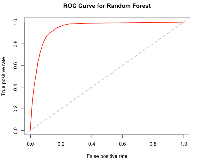
Figure 4 – ROC chart for Random Forest model
The final thing you can calculate is the Area Under the Curve (AUC). This is a measure of the area under the curve in Figure 4. This can be a very useful measure when comparing multiple models, as the model with the higher AUC value will typically be the optimal model.
#compute area under curve
auc <- performance(RF_pred,"auc")
auc <- unlist(slot(auc, "y.values"))
minauc<-min(round(auc, digits = 2))
maxauc<-max(round(auc, digits = 2))
minauct <- paste(c("min(AUC) = "),minauc,sep="")
maxauct <- paste(c("max(AUC) = "),maxauc,sep="")
minauct
[1] "min(AUC) = 0.94"
Summary
Random Forest is a powerful machine learning algorithm that allows you to create models that can give good overall accuracy with making new predictions. This is achieved because Random Forest is an ensemble machine learning technique that builds and uses many tens or hundreds of decision trees, all created in a slightly different way. Each of these decision trees is used to make a prediction for a new record, and a majority vote is done to determine the final predicted outcome. In this first article, the basics of Random Forest has been covered, along with how to build and use Random Forest models using the R language. In the second article [insert link here] examples will be given on how to use Random Forest using the Python language and how to use it in Oracle 18c Database.
Start the discussion at forums.toadworld.com