This tutorial applies to Toad Data Point 4.3 or later.
Summary
This tutorial demonstrates how to create a Toad Pivot Grid file and how to use Automation to refresh the pivot grid and generate a report.
In this tutorial you will learn:
- How to create a Toad Pivot Grid file
- How to use the Pivot Grid activity in Automation
You will need:
- A sample database
- A query to use for creating a pivot grid
Watch these videos for more information on how to use the Toad Pivot Grid:
Introduction
A pivot grid is a great way to display a summary of your data. Pivot grids are also great to use as reports. You can create a pivot grid in Toad and save it (with the query) as a Toad Pivot Grid file. You can also export the pivot grid to an Excel pivot table or an Excel grid, among other options.
In this tutorial you will create a pivot grid in Toad and then build an Automation script to refresh the pivot grid and generate an Excel report. The query provided in this tutorial is designed to be used with the Toad Sample Database (available with Toad Data Point). To follow along with a different sample database, use a query in which the result set can be summarized in a pivot grid.
Create a Toad Pivot Grid File
- To get started, connect to the Toad Sample Database.
- Select Tools | Editor to open a SQL Editor window. Or select Tools | Query Builder to use the Query Builder.
-
Enter your query in the Editor or Query Builder and execute it. To follow along using the Toad Sample Database, enter the following query:
SELECT ORDERS.ORDER_DATE, ORDERS.ORDER_ID, ORDER_ITEM.QUANTITY, ITEM.RETAIL_PRICE, CONTACT.FIRST_NAME,
CONTACT.LAST_NAME, REGION.REGION_NAME

FROM ORDERS ORDERS, ORDER_ITEM ORDER_ITEM, ITEM ITEM, CONTACT CONTACT, REGION REGION, ADDRESS ADDRESS
WHERE ORDERS.ORDER_ID = ORDER_ITEM.ORDER_ID
AND ORDER_ITEM.ITEM_ID = ITEM.ITEM_ID
AND ORDERS.CONTACT_ID = CONTACT.CONTACT_ID
AND CONTACT.ADDRESS_ID = ADDRESS.ADDRESS_ID
AND ADDRESS.REGION_ID = REGION.REGION_ID -
After the query executes, select the Pivot & Chart tab of the Results pane. Let’s build a quick pivot grid to preview the data before sending it to the Pivot Grid tool.
For more information about how to send data to the Pivot Grid tool or the Pivot & Chart tab, see Pivot and Chart Data.
-
Build the preview pivot grid by dragging fields from the Pivot Grid field list to the grid or to the Areas below the field list.
- Drag ORDER_DATE from the field list to the Column Area.
- Now drag REGION_NAME to the Row Area.
- Finally, drag QUANTITY to the Data Area.
Your pivot grid should look similar to the following screen shot. To display the bar graph, select Bar from the Type drop-down list. Click
 and clear Chart Selection Only to display all data.
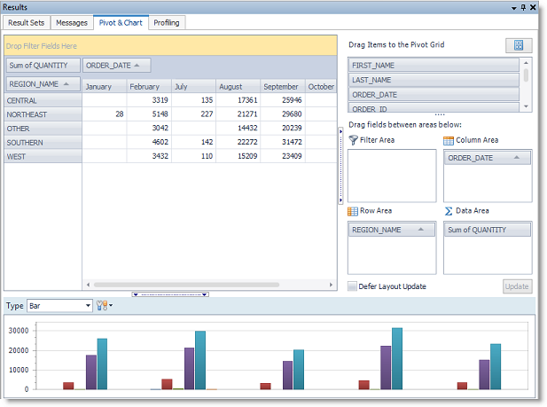
The Pivot & Chart tab of the Editor allows you to preview your data while you are working on a query. To save the pivot grid, you must send it to the Pivot Grid tool. This allows you to save the query and pivot layout as a Toad Pivot Grid file which can be used in an Automation script.
-
When you are satisfied that your query and result set produce the kind of pivoted data you want, right-click the pivot grid and select Move to Document.
When Toad prompts you to save the data with the query, select Yes. The query, data, and pivot grid layout are sent to the Pivot Grid tool which opens in a new window.
Tip: To start with a clean pivot grid, send only the query to the Pivot Grid tool. To do this, right-click the grid in the Result Sets tab and select Send To | Pivot Grid.
- The Pivot Grid window is similar to the Pivot & Chart tab. By default, the right pane contains a field list and a group of pivot grid destinations. The layout of this pane is similar to Excel and you can customize it by clicking
 .
. - You can edit the query at any time by clicking Edit Query in the upper-right corner. Use this dialog to modify the query or preview data.
- Let's start working with this pivot grid. Let’s add a calculated column.
-
Click
 in the Pivot Grid toolbar.
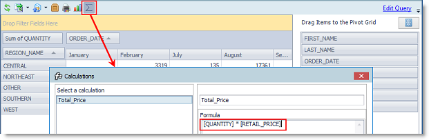
- In the Calculations dialog, enter "Total_Price" in the name field. Select Fields in the lower-left pane to display a list of columns in the right pane. Double-click QUANTITY to add it to the Formula field. Then click the X operator. Then double-click RETAIL_PRICE to create the formula “QUANTITY * RETAIL_PRICE.”
- The Calculations dialog provides a very useful feature that allows you to save an expression (formula) for reuse in other calculated columns. To use this feature, click Add As Saved Expression. The expression is added to the Saved Expressions list.
- Click OK to save your work and close the dialog.
-
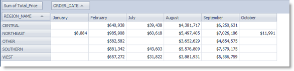
- Remove the QUANTITY field from the Data Area by dragging it back to the fields list. Now drag the Total_Price calculated field you just created to the Data Area. The result is a pivot grid showing total sales per region for each month.
-
Let's make sure the sales values display as currency. Right-click the data area in the pivot grid and select Value Field Settings. In the dialog click Number Format. Select Currency and click OK.
-
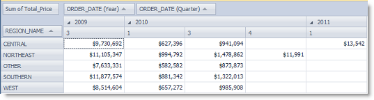
One very convenient feature of the pivot grid is the way it groups dates. To demonstrate this, right-click the ORDER_DATE field in the Column Area and select Group By. From the list, select Year. Then add the date column a second time and select Group By | Quarter.
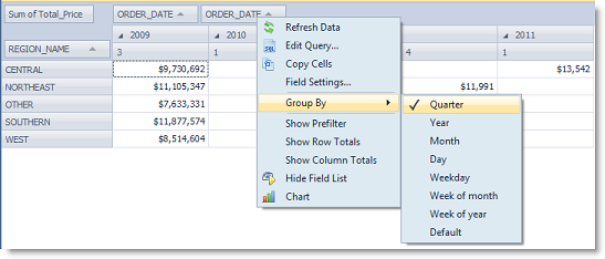
To make your report more meaningful, customize the field names. Right-click the second ORDER_DATE field and select Field Settings. Change the name to "ORDER_DATE (Quarter)." Repeat this process with the first field and change the name to "ORDER_DATE (Year)."
Review your pivot grid and notice how columns are now grouped by year and sub-grouped by quarter, as in the following example.
Tip: You can rename fields in the Data Area also. Right-click a data field or value and select Value Field Settings.
-
Filtering the Data. You may want to filter the data displayed in the pivot grid. You can filter by the field values in any field in your result set.
- Place your cursor over the REGION_NAME field (Row Area) and click
 . Select only Central and Southern. Click OK. Only data for the Central and Southern regions is displayed. The filter icon now displays in the field name to indicate that a filter is applied.
 - Click
 again and click the radio button and then select a region. The radio button allows you to ensure that only one value is selected at a time.
 - Click
 , click the radio button again to deselect it, and then select Show All.
 - Now remove the REGION_NAME field from the Row Area by dragging it back to the field list. Drag the LAST_NAME field to the Row Area. Your pivot now displays total price per customer for each quarter.
- You can also filter by a field not displayed in the pivoted data. Drag the REGION_NAME field to the Filter Area (upper-left corner of pivot grid). Click
 in the REGION_NAME field and select only the West region. The grid now displays data for only those customers located in the West.
To create a more complex filter based on more than one field, you can use a pre-filter. To do this, right-click the pivot grid and select Show Prefilter. After it is created, the pre-filter is displayed along the bottom of the pivot grid.
- Place your cursor over the REGION_NAME field (Row Area) and click
-
Inspecting the Data. In the pivot grid, locate the value (cell) for the customer named Austin in 2009, quarter 1. Double-click the value. This action drills down to the data behind the value and in this case reveals multiple first names. So, drag the FIRST_NAME field from the field list to the Row Area, making sure to place it below the LAST_NAME field (or to the right of it in the pivot grid). Field order determines grid layout.
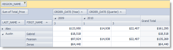
Tip: Right-click the pivot grid and select Show Column Totals to add a Grand Total column. Right-click the Grand Total column header to rename it.
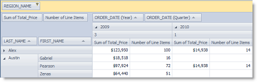
- A very useful feature of the pivot grid is the ability to add a duplicate field with a different aggregate type allowing you to display several different aggregates in one grid.
- If you have been following along, your grid Data Area contains the Total_Price field with the Sum aggregate type (which is the default) applied. Drag another Total_Price field to the Data Area.
-
Right-click the duplicate field and select Value Field Settings. In the Summarize Values By tab, select Count (deselect Sum). In the Custom Name field, enter “Number of Line Items” to distinguish this aggregate.
- Now add the QUANTITY field to the Data Area. Right-click this field and select Value Field Settings. Select Sum as the aggregate type. Change the name to “Total Items.” In the Show Values As tab, select No Calculation.
-
Add the QUANTITY field again using the same value field settings, except in the Show Values As tab, select % of Column Grand Total. Name this field "Total Items %."
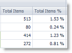
- The duplicate QUANTITY fields are used to demonstrate how duplicate fields allow you to view the same value, but using a different measurement. Remove the QUANTITY fields by dragging them back to the field list.
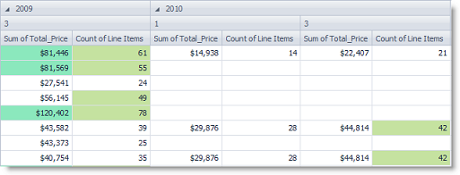
- Let's add some conditional formatting.
- Right-click a data value in the pivot grid and select Format Rules | Manage Rules.
- Click New Rule. Select the Format only top or bottom ranked values rule type. Then select Top and enter "25." Select % of column values.
- Click Format. Select the Fill tab and choose a light green fill. Click OK.
With conditional formatting, your pivot grid might look something like this.
- Now let's review the chart, a great way to visualize your pivoted data. Click
 to show the chart pane if it is not displayed.
- In the Type field, browse different chart types and then select one.
-
Click the arrow beside
 and select Chart Selection Only. Now select some cells in the pivot grid (use CTRL+Click to select multiple areas).
The chart displays only the data in the selected cells. This is a great way to visualize a subset of data from the pivot grid.
-
Before creating the Automation script, let's test the Excel output. You can export the pivot grid to a few different formats, including an Excel pivot table and an Excel grid. Note the following differences:
- Excel pivot table—In this format, the exported Excel file contains an Excel pivot table, as well as a sheet containing the underlying result set.
- Excel grid—In this format, the exported Excel file contains the summarized data as a data set. Only the data in the pivot grid is exported. This format presents full rows of data wherever the pivot grid grouped data into merged cells.
For this tutorial, let's export to an Excel pivot table.
- Click
 and select Excel Pivot. In the Export dialog, select a file name and location. To learn more about the options available in the Export dialog, see Specify Excel Export Options. Click OK to begin exporting.
 - Open the exported Excel file when prompted. Review the pivot table. The second sheet contains the underlying data. At this point, you can return to the Toad pivot grid window and modify the pivot grid or the query and re-export until you are satisfied with the results.
-
After you have configured the Toad pivot grid to your satisfaction, save the file as a Toad Pivot Grid file (.tpg). You will use this file in your Automation script.
When Toad prompts you to save the data with the query, select Yes to save the data. When you open the file again, you must manually refresh the query to access the latest data. To force a refresh upon opening the file, select No.
Create Script
- Select Tools | Automation to open a new Automation window.
- Click the Toad Pivot Grid activity to add it to the Automation design window.
- In the Activity Input tab, click
 in the Pivot file field and browse to and select the Toad Pivot Grid file you just created.
 -
In the Export to File section, for this tutorial select Excel Pivot as the export type. This option allows you to export both the pivot grid and the underlying data to an Excel pivot table file. The exported file includes an Excel pivot table and the result set. Then enter a file name and location for your export file.
Click Export options to customize the Excel file. See Specify Excel Export Options for more information about selecting Excel file options.
Tip: You can export to other destinations and file types. See Use Database Automation Activities for more information about other actions available with the Toad Pivot Grid Automation activity.
-
Click Run to save and run your script.
The script opens the existing Toad Pivot Grid file, executes the query, and exports the data to the Excel pivot table file.
- After the script executes, review the Log. Click the hyperlink to view the Excel output file.
Use Toad Pivot Grid files as a convenient way to keep your SQL query with your pivot grid. And then use Automation to automatically refresh your pivot grid and generate a report.
Schedule A Script
See Schedule Your Script to learn how to schedule the Automation script.
How to get the most out of Toad Data PointToad Data Point, is a powerful tool that will help you access and prepare data for faster business insights. Toad Data Point enables business or data analysts to seamlessly access more than 50 data sources—both on premises and in the cloud—and switch between these data sources with near-zero transition times. Users can connect, query and prepare data for faster business insights. Whether you are currently a Toad Data Point customer or just getting started with our free 30-day trial, learn more and access the Toad Data Point User Guide. If you're in a trial and Toad Data Point is helping you access and prepare data for faster business insights, buy it now or contact a sales representative. |
Useful resources
Webinar series: Data Preparation Made Easy: Toad Data Point Webcast Series
Video: Top 5 reasons to buy Toad Data Point Professional Edition, a solution for simplifying data access, integration, and provisioning.
Case study #1: Dell: Enterprise financial group solves data prep challenge.
Case study #2: Opening doors and creating opportunities with data insights.
Related articles
Forum: How to transpose rows to columns
Blog: Access more Toad Data Point blogs
Got questions?
If you have any questions, please post questions to the Toad Data Point forum on Toad World.
Start the discussion at forums.toadworld.com