I. Introduction
In the IT industry we go through a tedious and long process of acquiring infrastructure (hardware software and licenses). Typically, projects are held back due to infrastructure delays in definition, contracts, support and licenses. Oftentimes, projects have been cancelled due to the infrastructure cost and non-ability of escalation. Cloud computing addresses all these difficulties and more. Teams now can focus in more important aspects of the projects: business, functionalities, and applications; and pay little heed to the infrastructure, which is totally or partially managed by the cloud provider. Everything from storage for petabytes of data to high compute capacity is at your disposals. You have the software, hardware, all on demand and at your disposals everywhere and anytime, with the ability to scale, and at lower cost.
This article is the second in a series on Big Data in the cloud. In it, we will continue introducing the Big Data warehouse service in AWS. In the first article, we explained the Redshift architecture and setup a cluster. Now we will focus on the database design and good practices to maximize the usage of the Big Data Warehouse service in the cloud.
II. Amazon Redshift Database Creation
Amazon Redshift is a container composed of one or more databases. The database is where you create the users and tables and run queries. You use the CREATE DATABASE command to create a database. You may specify options like CONNECTION LIMIT, which is the maximum number of database connections users are permitted to have open concurrently, and database owner. There are some restrictions with CREATE DATABASE:
– Maximum of 60 user-defined databases per cluster.
– Maximum of 127 bytes for a database name.
– Cannot be a reserved word.
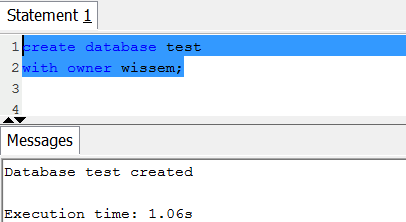
Example: The following example creates a database named test and gives ownership to the user wissem:
You can Query the PG_DATABASE_INFO catalog table. The catalog PG_DATABASE_INFO stores information about the available databases.
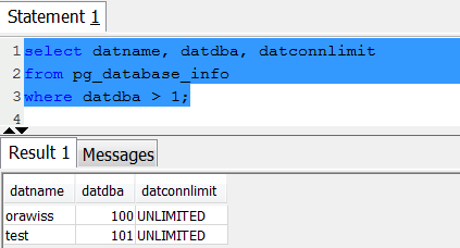
The following table describes every column used in the query.
|
Name |
Description |
|
datname |
Database name |
|
datdba |
Owner of the database, usually the user who created it |
|
datconnlimit |
Sets maximum number of concurrent connections that can be made to this database. |
III. Amazon Redshift Database User Creation
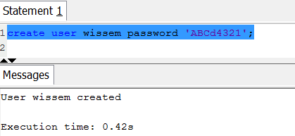
By default, only the master user that you created when you launched the cluster has access to the initial database in the cluster. To grant other users access, you must create one or more user accounts. Database user accounts are global across all the databases in a cluster; they do not belong to individual databases. Use the CREATE USER command to create a new database user.
Example:
IV. Amazon Redshift Table Design
You can create a table using the CREATE TABLE command. This command specifies the name of the table, the columns, and their data types. In addition to columns and data types, the Amazon Redshift CREATE TABLE command also supports specifying compression encodings, distribution strategy, and sort keys. These CREATE TABLE options are keys for query performance.
1- Data types
Amazon Redshift columns support:
- Numeric data types; SMALLINT, INTEGER, BIGINT, DECIMAL, REAL (FLOAT4), DOUBLE PRECISION (FLOAT8)
- Character data Types: CHAR, VARCHAR
- Boolean; BOOLEAN
- Date data types: DATE, TIMESTAMP, TIMESTAMPTZ
2- Compression Encoding
Data compression is one of the query performance factors in a Redshift Cluster. You can specify compression encoding on a per-column basis as part of the CREATE TABLE command.
The following Compression encodings are supported:
- BYTEDICT
- DELTA
- DELTA32K
- LZO
- MOSTLY8
- MOSTLY16
- MOSTLY32
- RAW (no compression, the default setting)
- RUNLENGTH
- TEXT255
- TEXT32K
- ZSTD
3- Distribution Styles
During the first load of data into a table, the cluster distributes the rows according to the distribution style. All the compute nodes participate in parallel query execution, working on data that is distributed across the slices. You should assign distribution styles to achieve the following goals:
– Minimize the data movement between compute nodes by placing the rows from joining tables and the rows for joining columns on the same slices.
– Equally distribute data among the slices in a cluster so the workload can be allocated equally to all the slices.
When you create a table, you designate one of three distribution styles: KEY, ALL, or EVEN. More details can be found in the documentation: http://docs.aws.amazon.com/redshift/latest/dg/c_choosing_dist_sort.html
– KEY distribution: The rows are distributed according to the values in one column. The leader node will attempt to place matching values on the same node slice.
– ALL distribution: A copy of the entire table is distributed to every node.
– EVEN distribution: The rows are distributed across the slices in a round-robin fashion, regardless of the values in any particular column. EVEN distribution is the default distribution style.
HINT: Use the EXPLAIN command to analyze the redistribution steps in the SQL query plan. When looking into explain plan, try to reduce or eliminate the DS_BCAST_INNER and DS_DIST_BOTH operations. DS_BCAST_INNER indicates that the inner join table was broadcast (copied) to every slice. A DS_DIST_BOTH would indicate that both the outer join table and the inner join table were redistributed across the slices. Broadcasting and redistribution can be expensive steps in terms of execution cost.
4- Sort Keys
At table creation, you may specify one or more sort key columns. When data is initially loaded into the empty table, the rows are stored on disk in sorted order. Information about sort key columns is passed to the query planner, and the planner uses this information to construct plans passed to every compute node. You can use either the INTERLEAVED or COMPOUND keyword with your CREATE TABLE or CREATE TABLE AS statement.
– A compound sort key, which is a subset of the sort key columns in order of the sort keys, is most useful when a query's filter applies conditions, such as filters and joins, that use a prefix. The performance degrades when queries depend only on secondary sort columns, without referencing the primary columns. COMPOUND is the default sort type.
– An interleaved sort key gives equal weight to each columns or subset of columns in the sort key. If multiple queries use different columns for filters, then you can often improve performance for those queries by using an interleaved sort style. When a query uses restrictive predicates on secondary sort columns, interleaved sorting significantly improves query performance as compared to compound sorting.
Refer to the documentation link: http://docs.aws.amazon.com/redshift/latest/dg/t_Sorting_data.html for more details about sort keys.
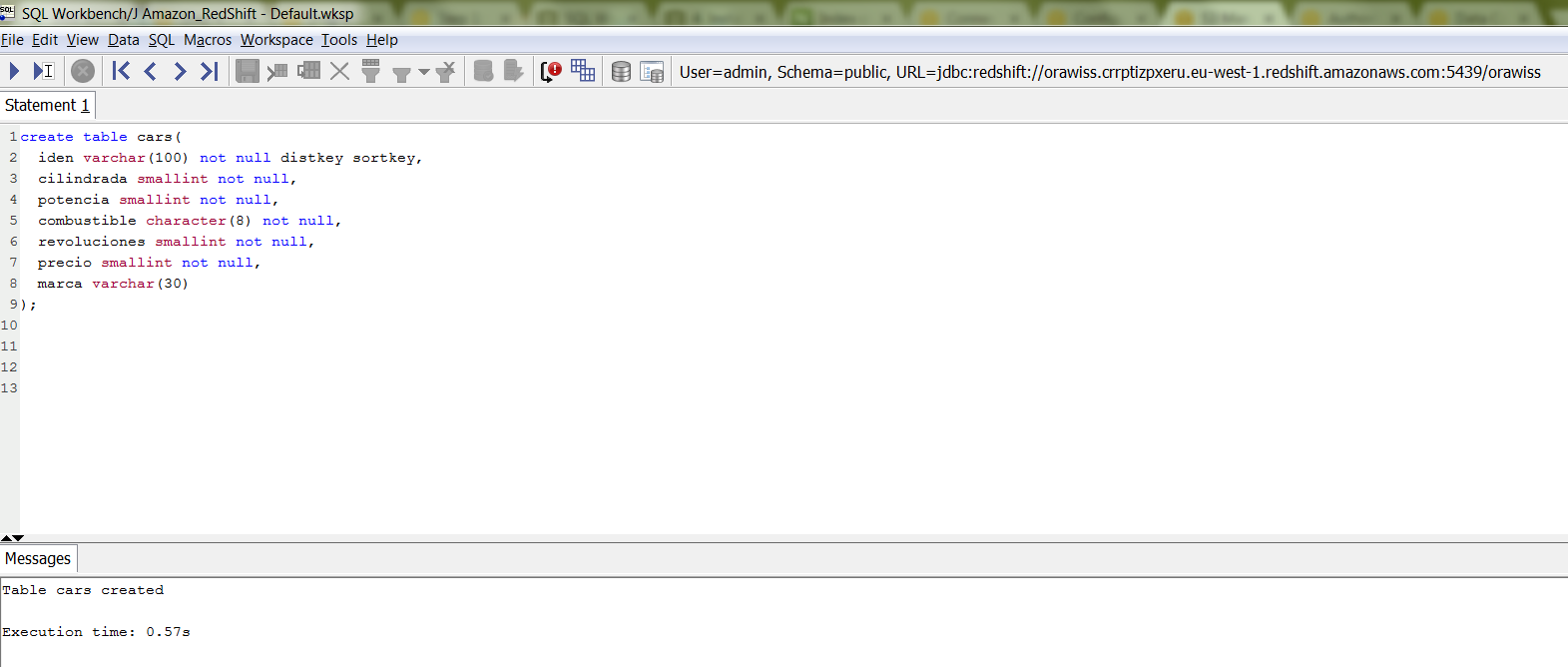
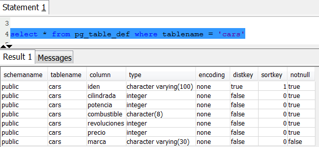
Example: In the following example we create a table called cars; which we will use later to load data into.
Query the pg_table_def system table to check the cars table definition.
5- Data Loading and Unloading
Amazon Redshift offers bulk loading data from multiple files stored in Amazon S3. The COPY command reads the data from input files and distributes it to the compute nodes in parallel. VACUUM and ANALYZE commands are recommended after every bulk load to reorganize the physical storage and update the system table statistics.
The ANALYZE command collects statistics about the contents of tables in the database and stores the results in the pg_statistic system catalog. The query planner uses these statistics to help determine the most efficient execution plans for queries. With no parameter, ANALYZE examines every table in the current database. With a parameter, ANALYZE examines only that table. It is further possible to give a list of column names, in which case only the statistics for those columns are collected.
Data can also be exported outside the Amazon Redshift cluster using the UNLOAD command. This command can be used to generate delimited text files and store them in Amazon S3.
An important step to allow the COPY operation is to create an IAM role with Amazon S3 read only access policy attached to it.
You need first to create the IAM role like shown in the following screen; We called the IAM role: RedshiftCopyUnload
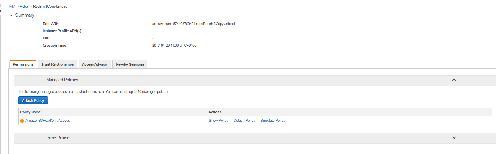
Take a note of the role ARN which will be supplied during the run of the COPY command.
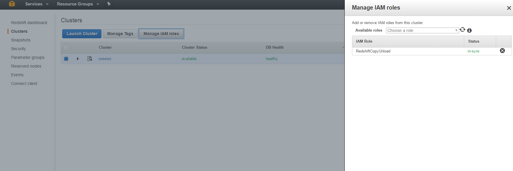
Once the IAM role RedshiftCopyUnload is created, you need to attach it to the Amazon Redshift cluster as shown in the following screen:
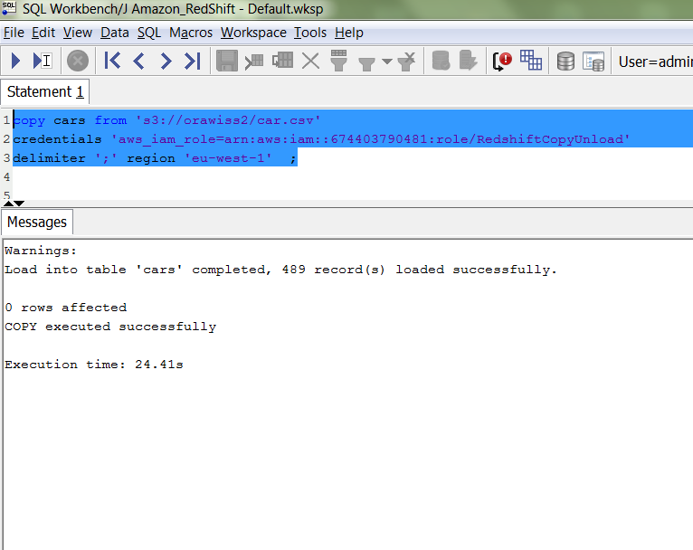
A prerequisite: Prior running the COPY command, the files must be present in the S3 bucket. Now, you can run the COPY command, to load the CSV file from the Amazon S3 into the cars table inside the Redshift cluster database. Note here we specified the region eu-west-1 is where the cluster is running.
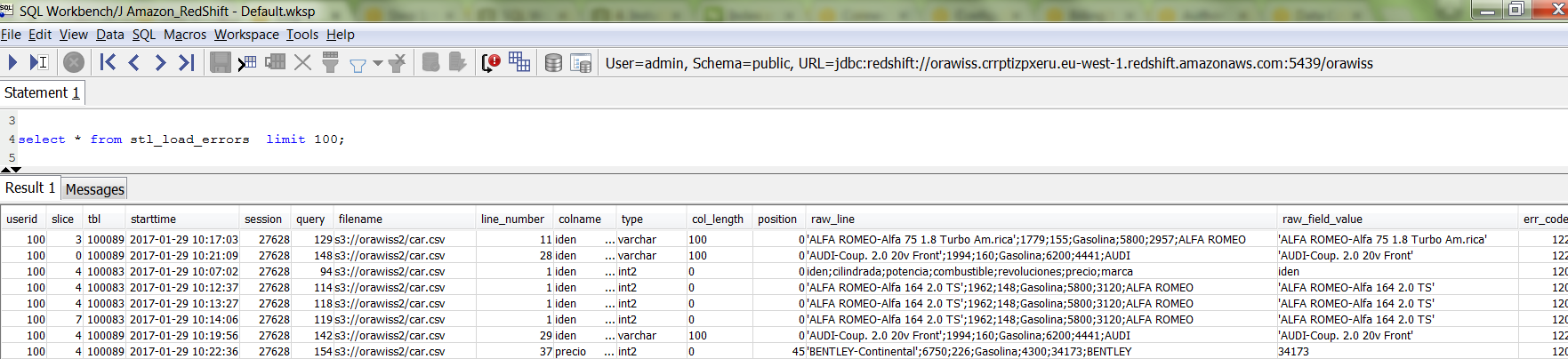
Query the table stl_load_errorsto check for any errors during the COPY command.
6- Querying Data
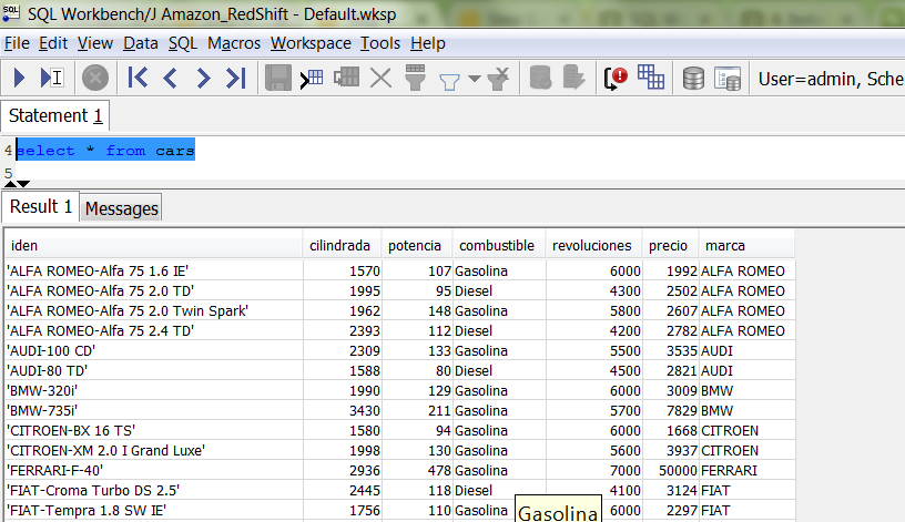
The Amazon Redshift SELECT returns rows from tables, views, and user-defined functions. Let’s query the cars table we created previously.
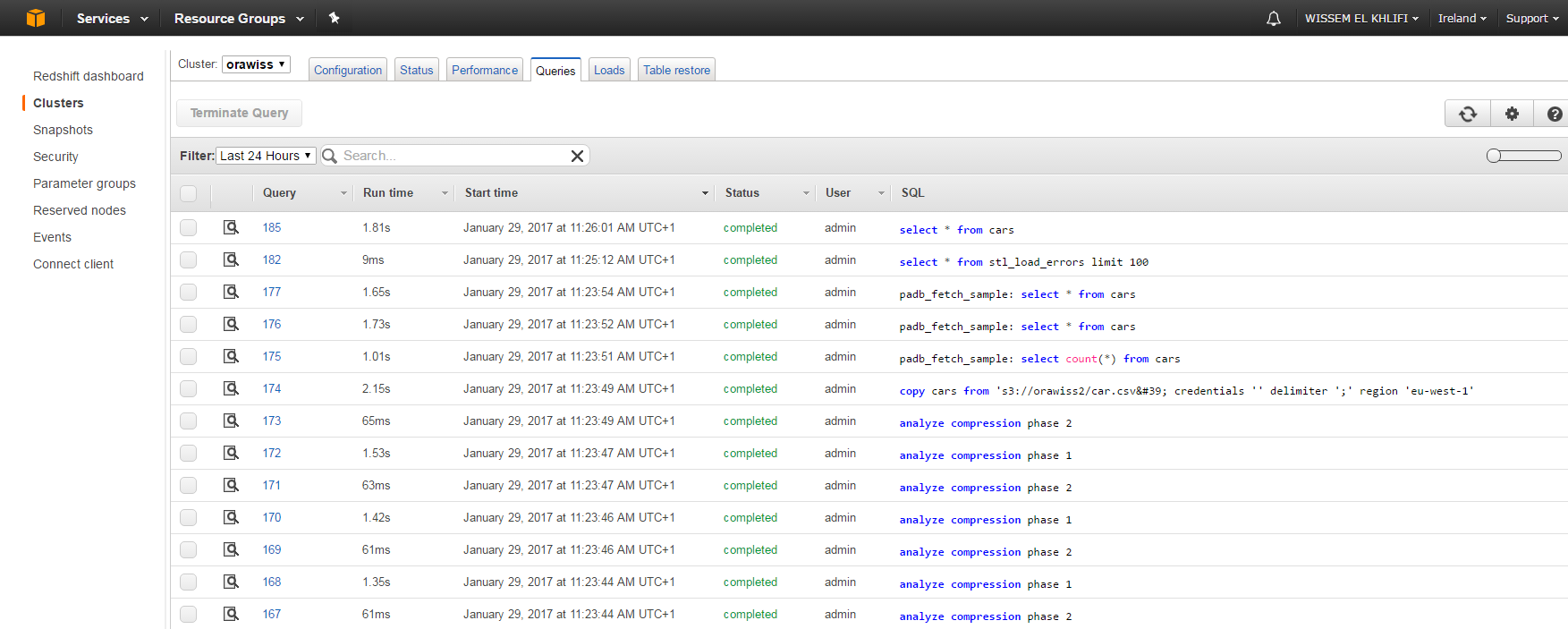
Sign in to the AWS Management Console and open the Amazon Redshift console at https://console.aws.amazon.com/redshift/.
In the cluster list in the right pane, choose orawiss for cluster name. Then choose the Queries tab.
The console displays list of queries you executed as shown in the example below.
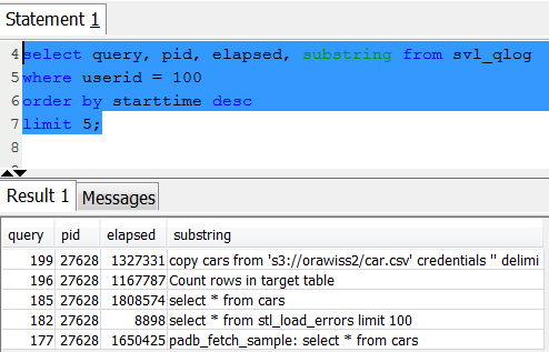
Alternatively, you can use the SQL tool to check the list of queries run in the Redshift database; You query the svl_qlog system table:
7- Query Plan
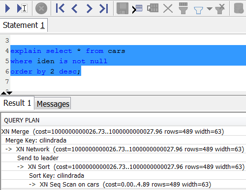
You can use the query plan to get information on every single operation required to execute a query. To create a query plan, run the EXPLAIN command followed by the actual query text. The query plan gives you the following information:
– Sort Key: Evaluates the ORDER BY clause, issued on cilindrada column.
– XN network; the Network operator sends the results to the leader node, where the Merge operator produces the final sorted results.
– Merge: Produces final sorted results of a query based on intermediate sorted results derived from operations performed in parallel.
– Check the documentation http://docs.aws.amazon.com/redshift/latest/dg/c-the-query-plan.html for more details about query plan in Amazon Redshift database.
V. Conclusion
In this article we introduced the Amazon Redshift database design and query performance; we have seen the simplicity and power of the Big Data Warehouse service in the Amazon Cloud. In future articles we will explore other Big Data services in the cloud.
Start the discussion at forums.toadworld.com